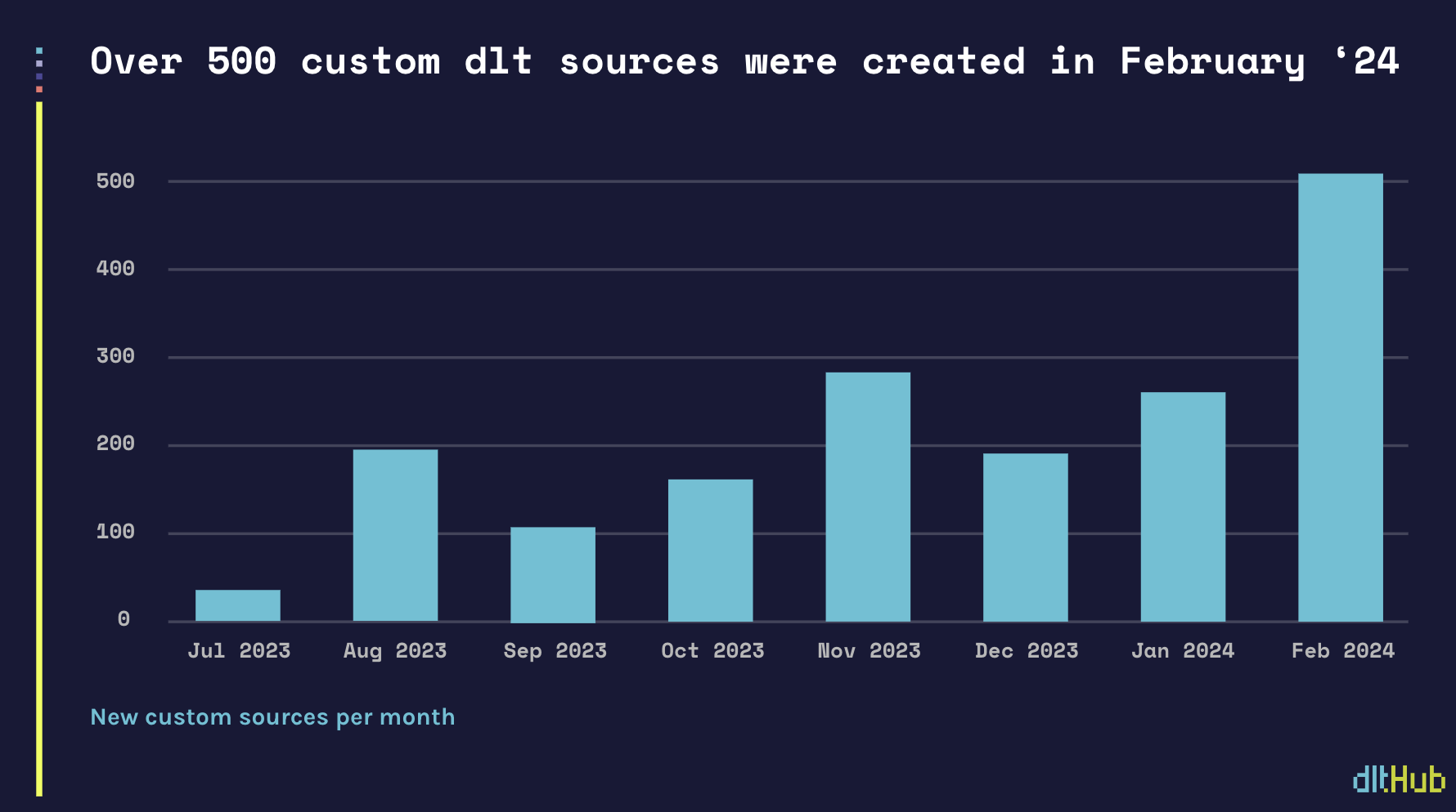
Celebrating over 500 ad hoc custom sources written by thedltcommunity in February
Today it is easier to pip install dlt and write a custom source than to setup and configure a traditional ETL platform.
The wider community is increasingly noticing these benefits. In February the community wrote over 500 dlt custom sources. Last week we crossed 2000 dlt total custom sources created since we launched dlt last summer.
A custom dlt source is something new for our industry. With dlt we automated the majority of the work data engineers tasks that are usually done in traditional ETL platforms. Hence, creating an ad hoc dlt pipeline and source is a dramatically simpler. Maintaining a custom dlt source in production is relatively easy as most of the common pipeline maintenance issues are handled.
How to get to 50,000 sources: let’s remove the dependency on source catalogs and move forward to ad hoc code
We think that “Pip install ETLs” or “EL as code” tools such as dlt are ushering a new era of ad hoc code. ad hoc code allows for automation and customization of very specific tasks.
Most of the market today is educated by Saas ETLs on the value of “source”/”connector” catalogs. The core is a short-tail catalog market of +-20 sources (product database replication, some popular CRMs and ads APIs) with the highest profit margins and intense competition among vendors. The long-tail source catalog market, depending on the vendor, is usually up to 400 sources, with much smaller support.
We think that source catalogs will become more and more irrelevant in the era of LLMs and ad hoc code. “EL as code” allows users to work with source catalog. From the beginning the dlt community has been writing wrappers for taps/connectors from other vendors, usually to migrate to a dlt pipeline at some point, as we documented in the customer story how Harness adopted dlt.
Even for short-tail, high quality catalog sources “EL as code” allows for fixes of hidden gotchas and customisation that makes data pipelines production-ready.
We also believe that these are all early steps in “EL as code”. Huggingface hosts over 116k datasets as of March ‘24. We at dltHub think that the ‘real’ Pythonic ETL market is a market of 100k of APIs and millions of datasets.
dlt has been built for humans and LLMs from the get go and this will make coding data pipelines even faster
Since the inception of dlt, we have believed that the adoption dltamong the next generation of Python users will depend on its compatibility with code generation tools, including Codex, ChatGPT, and any new tools that emerge on the market..
We have not only been building dlt for humans, but also LLMs.
Back in March ‘23 we released dlt init as the simplest way to add a pipeline/initialize a project in dlt. We rebuilt the dlt library in such a way that it performs well with LLMs. At the end of May ‘23 we opened up our dltHub Slack to the broader community.
However, it takes a long time to go from a LLM PoC to production-grade code. We know much of our user base is already using ChatPGT and comparable tools to generate sources. We hear our community's excitement about the promise of LLMs for this task. The automation promise is in both in building and configuring pipelines. Anything seems possible, but if any of you have played around this task with ChatPGT - usually the results are janky. Along these lines in the last couple of months we have been dog fooding the PoC that can generate dlt pipelines from an OpenAPI specification.
We think that at this stage we are a few weeks away from releasing our next product that makes coding data pipelines faster than renting connector catalog: a dlt code generation tool that allows dlt users create datasets from the REST API in the coming weeks.
TL;DR: This blog post introduces a cost-effective solution for event streaming that results in up to 18x savings. The solution leverages Cloud Pub/Sub and DLT to build an efficient event streaming pipeline.
Event tracking is a complicated problem for which there exist many solutions. One such solution is Segment, which offers ample startup credits to organizations looking to set up event ingestion pipelines. Segment is used for a variety of purposes, including web analytics.
note
💡 With Segment, you pay 1-1.2 cents for every tracked users.
Let’s take a back-of-napkin example: for 100.000 users, ingesting their events data would cost $1000.
The price of $1000/month for 100k tracked users doesn’t seem excessive, given the complexity of the task at hand.
However, similar results can be achieved on GCP by combining different services. If those 100k users produce 1-2m events, those costs would stay in the $10-60 range.
In the following sections, we will look at which GCP services can be combined to create a cost-effective event ingestion pipeline that doesn’t break the bank.
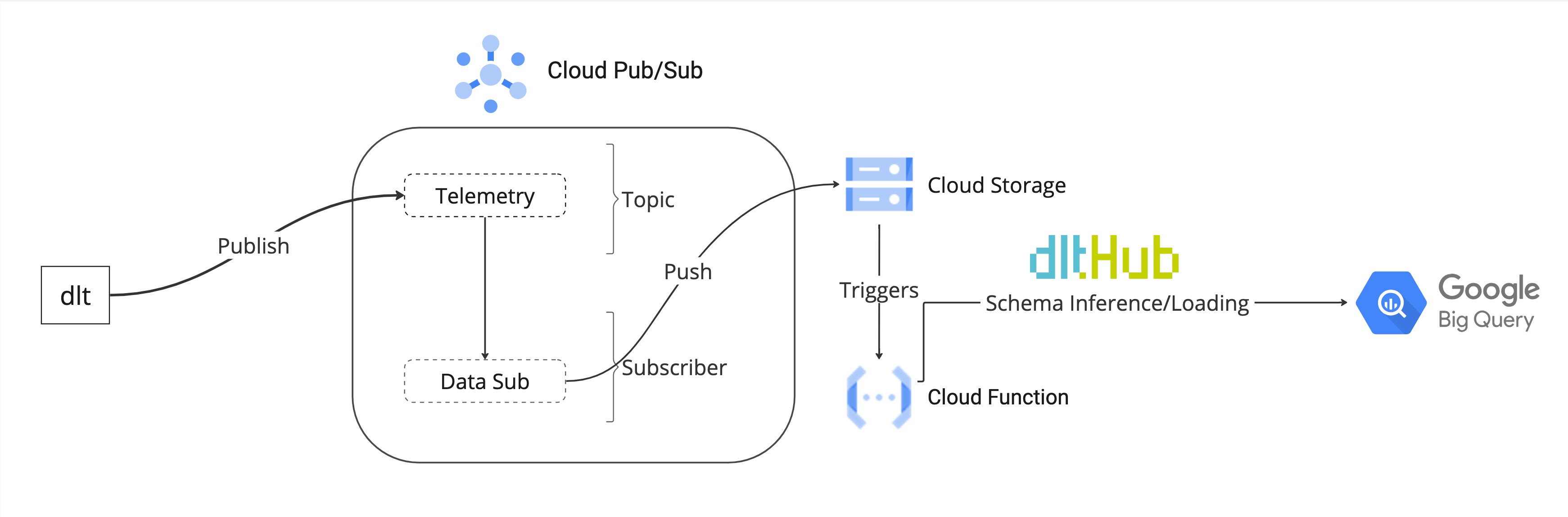
Our proposed solution to replace Segment involves using dlt with Cloud Pub/Sub to create a simple, scalable event streaming pipeline. The pipeline's overall architecture is as follows:
In this architecture, a publisher initiates the process by pushing events to a Pub/Sub topic. Specifically, in the context of dlt, the library acts as the publisher, directing user telemetry data to a designated topic within Pub/Sub.
A subscriber is attached to the topic. Pub/Sub offers a push-based subscriber that proactively receives messages from the topic and writes them to Cloud Storage. The subscriber is configured to aggregate all messages received within a 10-minute window and then forward them to a designated storage bucket.
Once the data is written to the Cloud Storage this triggers a Cloud Function. The Cloud Function reads the data from the storage bucket and uses dlt to ingest the data into BigQuery.
This section dives into a comprehensive code walkthrough that illustrates the step-by-step process of implementing our proposed event streaming pipeline.
Implementing the pipeline requires the setup of various resources, including storage buckets and serverless functions. To streamline the procurement of these resources, we'll leverage Terraform—an Infrastructure as Code (IaC) tool.
Next, we focus on establishing the necessary permissions for our pipeline. A crucial step involves creating service account credentials, enabling Terraform to create and manage resources within Google Cloud seamlessly.
Please refer to the Google Cloud documentation here to set up a service account. Once created, it's important to assign the necessary permissions to the service account. The project README lists the necessary permissions. Finally, generate a key for the created service account and download the JSON file. Pass the credentials as environment variables in the project root directory.
Within this structure, the Terraform directory houses all the Terraform code required to set up the necessary resources on Google Cloud.
Meanwhile, the cloud_functions folder includes the code for the Cloud Function that will be deployed. This function will read the data from storage and use dlt to ingest data into BigQuery. The code for the function can be found in cloud_functions/main.py file.
To begin, integrate the service account credentials with Terraform to enable authorization and resource management on Google Cloud. Edit the terraform/main.tf file to include the path to your service account's credentials file as follows:
Next, in the terraform/variables.tf define the required variables. These variables correspond to details within your credentials.json file and include your project's ID, the region for resource deployment, and any other parameters required by your Terraform configuration:
We are now ready to set up some cloud resources. To get started, navigate into the terraform directory and terraform init. The command initializes the working directory containing Terraform configuration files.
With the initialization complete, you're ready to proceed with the creation of your cloud resources. To do this, run the following Terraform commands in sequence. These commands instruct Terraform to plan and apply the configurations defined in your .tf files, setting up the infrastructure on Google Cloud as specified.
terraform plan
terraform apply
This terraform plan command previews the actions Terraform intends to take based on your configuration files. It's a good practice to review this output to ensure the planned actions align with your expectations.
After reviewing the plan, execute the terraform apply command. This command prompts Terraform to create or update resources on Google Cloud according to your configurations.
The following resources are created on Google Cloud once terraform apply command is executed:
Name
Type
Description
tel_storage
Bucket
Bucket for storage of telemetry data.
pubsub_cfunctions
Bucket
Bucket for storage of Cloud Function source code.
storage_bigquery
Cloud Function
The Cloud Function that runs dlt to ingest data into BigQuery.
telemetry_data_tera
Pub/Sub Topic
Pub/Sub topic for telemetry data.
push_sub_storage
Pub/Sub Subscriber
Pub/Sub subscriber that pushes data to Cloud Storage.
Now that our cloud infrastructure is in place, it's time to activate the event publisher. Look for the publisher.py file in the project root directory. You'll need to provide specific details to enable the publisher to send events to the correct Pub/Sub topic. Update the file with the following:
The publisher.py script is designed to generate dummy events, simulating real-world data, and then sends these events to the specified Pub/Sub topic. This process is crucial for testing the end-to-end functionality of our event streaming pipeline, ensuring that data flows from the source (the publisher) to our intended destinations (BigQuery, via the Cloud Function and dlt). To run the publisher execute the following command:
Once the publisher sends events to the Pub/Sub Topic, the pipeline is activated. These are asynchronous calls, so there's a delay between message publication and their appearance in BigQuery.
The average completion time of the pipeline is approximately 12 minutes, accounting for the 10-minute time interval after which the subscriber pushes data to storage plus the Cloud Function execution time. The push interval of the subscriber can be adjusted by changing the max_duration in pubsub.tf
On average the cost for our proposed pipeline are as follows:
100k users tracked on Segment would cost $1000.
1 million events ingested via our setup $37.
Our web tracking user:event ratio is 1:15, so the Segment cost equivalent would be $55.
Our telemetry device:event ratio is 1:60, so the Segment cost equivalent would be $220.
So with our setup, as long as we keep events-to-user ratio under 270, we will have cost savings over Segment. In reality, it gets even better because GCP offers a very generous free tier that resets every month, where Segment costs more at low volumes.
GCP Cost Calculation:
Currently, our telemetry tracks 50,000 anonymized devices each month on a 1:60 device-to-event ratio. Based on these data volumes we can estimate the cost of our proposed pipeline.
Cloud Functions is by far the most expensive service used by our pipeline. It is billed based on the vCPU / memory, compute time, and number of invocations.
note
💡 The cost of compute for 512MB / .333vCPU machine time for 1000ms is as follows
Metric
Unit Price
GB-seconds (Memory)
$0.000925
GHz-seconds (vCPU)
$0.001295
Invocation
$0.0000004
Total
0.0022
This puts the monthly cost of ingesting 1 million events with Cloud Functions at:
Event streaming pipelines don’t need to be expensive. In this demo, we present an alternative to Segment that offers up to 18x in savings in practice. Our proposed solution leverages Cloud Pub/Sub and dlt to deliver a cost-effective streaming pipeline.
Following this demo requires knowledge of the publisher-subscriber model, dlt, and GCP. It took about 4 hours to set up the pipeline from scratch, but we went through the trouble and set up Terraform to procure infrastructure.
Use terraform apply to set up the needed infrastructure for running the pipeline. This can be done in 30 minutes, allowing you to evaluate the proposed solution's efficacy without spending extra time on setup. Please do share your feedback.
P.S: We will soon be migrating from Segment. Stay tuned for future posts where we document the migration process and provide a detailed analysis of the associated human and financial costs.
At dltHub, we have been pioneering the future of data pipeline generation, making complex processes simple and scalable. We have not only been building dlt for humans, but also LLMs.
Pipeline generation on a simple level is already possible directly in ChatGPT chats - just ask for it. But doing it at scale, correctly, and producing comprehensive, good quality pipelines is a much more complex endeavour.
Our early exploration with code generation
As LLMs became available at the end of 2023, we were already uniquely positioned to be part of the wave. By being a library, a LLM could use dlt to build pipelines without the complexities of traditional ETL tools.
This raised from the start the question - what are the different levels of pipeline quality? For example, how does a user code snippet, which formerly had value, compare to LLM snippets which can be generated en-masse? What does a perfect pipeline look like now, and what can LLMs do?
We were only able to answer some of these questions, but we had some concrete outcomes that we carry into the future.
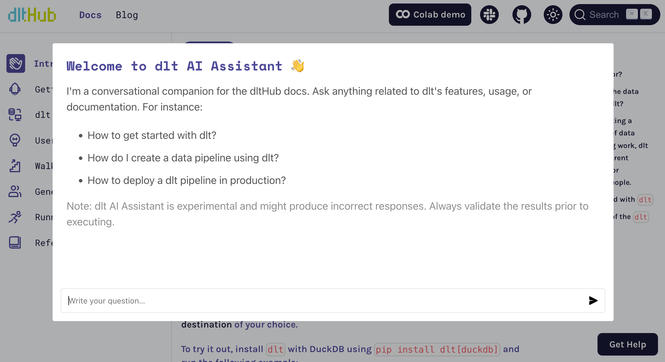
In June ‘23 we added a GPT-4 docs helper that generates snippets
try it on our docs; it's widely used as code troubleshooter
OpenApi spec describes the api; Just as we can create swagger docs or a python api wrapper, we can create pipelines
Running into early limits of LLM automation: A manual last mile is needed
Ideally, we would love to point a tool at an API or doc of the API, and just have the pipeline generated.
However, the OpenApi spec does not contain complete information for generating a complete pipeline. There’s many challenges to overcome and gaps that need to be handled manually.
While LLM automation can handle the bulk, some customisation remains manual, generating requirements towards our ongoing efforts of full automation.
The dlt community has been growing steadily in recent months. In February alone we had a 25% growth on Slack and even more in usage.
New users generate a lot of questions and some of them used our onboarding program, where we speed-run users through any obstacles, learning how to make things smoother on the dlt product side along the way.
Onboarding usually means building a pipeline POC fast
During onboarding, most companies want to understand if dlt fits their use cases. For these purposes, building a POC pipeline is pretty typical.
This is where code generation can prove invaluable - and reducing a build time from 2-3d to 0.5 would lower the workload for both users and our team.
💡 To join our onboarding program, fill this form to request a call.
Case Study: How our solution engineer Violetta used our PoC to generate a production-grade Chargebee pipeline within hours
In a recent case, one of our users wanted to try dlt with a source we did not list in our public sources - Chargebee.
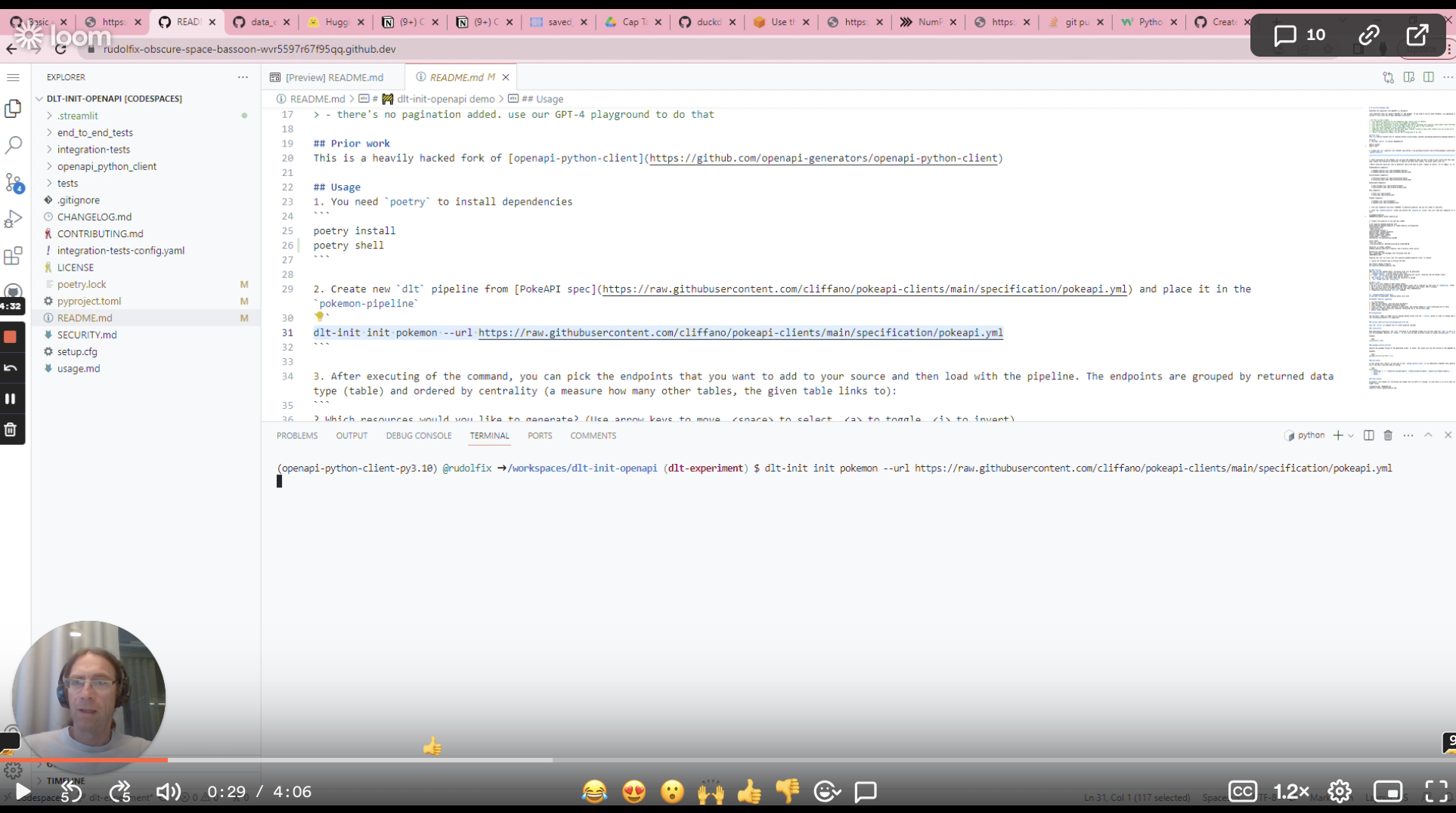
Since the Chargebee API uses the OpenAPI standard, we used the OpenAPI PoC dlt pipeline code generator that we built last year.
So the first thing I found extremely attractive — the code generator actually created a very simple and clean structure to begin with.
I was able to understand what was happening in each part of the code. What unfortunately differs from one API to another — is the authentication method and pagination. This needed some tuning. Also, there were other minor inconveniences which I needed to handle.
There were no great challenges. The most difficult tedious probably was to manually change pagination in different sources and rename each table.
1) Authentication
The provided Authentication was a bit off. The generated code assumed the using of a username and password but what was actually required was — an empty username + api_key as a password. So super easy fix was changing
Also I was pleasantly surprised that generator had several different authentication methods built in and I could easily replace BasicAuth with BearerAuth of OAuth2 for example.
2) Pagination
For the code generator it’s hard to guess a pagination method by OpenAPI specification, so the generated code has no pagination 😞. So I had to replace a line
The code wouldn’t run because it wasn’t able to find some models. I found a commented line in generator script
# self._build_models()
I regenerated code with uncommented line and understood why it was commented. Code created 224 .py files under the models directory. Turned out I needed only two of them. Those were models used in api code. So I just removed other 222 garbage files and forgot about them.
4) Namings
The only problem I was left with — namings. The generated table names were like
ListEventsResponse200ListItem or ListInvoicesForACustomerResponse200ListItem . I had to go and change them to something more appropriate like events and invoices .
I did a walk-through with our user. Some additional context started to appear. For example, which endpoints needed to be used with replace write disposition, which would require specifying the merge keys. So in the end this source would still require some testing to be performed and some fine-tuning from the user.
I think the silver lining here is how to start. I don’t know how much time I would’ve spent on this source if I started from scratch. Probably, for the first couple of hours, I would be trying to decide where should the authentication code go, or going through the docs searching for information on how to use dlt configs. I would certainly need to go through all API endpoints in the documentation to be able to find the one I needed. There are a lot of different things which could be difficult especially if you’re doing it for the first time.
I think in the end if I had done it from scratch, I would’ve got cleaner code but spent a couple of days. With the generator, even with finetuning, I spent about half a day. And the structure was already there, so it was overall easier to work with and I didn’t have to consider everything upfront.
We are currently working on making full generation a reality.
Here at dltHub, we work on the python library for data ingestion. So when I heard from Airbyte that they are building a library, I was intrigued and decided to investigate.
What is PyAirbyte?
PyAirbyte is an interesting Airbyte’s initiative - similar to the one that Meltano had undertook 3 years ago. It provides a convenient way to download and install Airbyte sources and run them locally storing the data in a cache dataset. Users are allowed to then read the data from this cache.
A Python wrapper on the Airbyte source is quite nice and has a feeling close to Alto. The whole process of cloning/pip installing the repository, spawning a separate process to run Airbyte connector and read the data via UNIX pipe is hidden behind Pythonic interface.
Note that this library is not an Airbyte replacement - the loaders of Airbyte and the library are very different. The library loader uses pandas.to_sql and sql alchemy and is not a replacement for Airbyte destinations that are available in Open Source Airbyte
Questions I had, answered
Can I run Airbyte sources with PyAirbyte? A subset of them.
Can I use PyAirbyte to run a demo pipeline in a colab notebook? Yes.
Would my colab demo have a compatible schema with Airbyte? No.
Is PyAirbyte a replacement for Airbyte? No.
Can I use PyAirbyte to develop or test during development Airbyte sources? No.
Can I develop pipelines with PyAirbyte? no
In conclusion
In wrapping up, it's clear that PyAirbyte is a neat little addition to the toolkit for those of us who enjoy tinkering with data in more casual or exploratory settings. I think this is an interesting initiative from Airbyte that will enable new usage patterns.
In large organisations, there are often many data teams that serve different departments. These data teams usually cannot agree where to run their infrastructure, and everyone ends up doing something else. For example:
40 generated GCP projects with various services used on each
Native AWS services under no particular orchestrator
That on-prem machine that’s the only gateway to some strange corporate data
and of course that SaaS orchestrator from the marketing team
together with the event tracking lambdas from product
don’t forget the notebooks someone scheduled
So, what’s going on? Where is the data flowing? what data is it?
The case at hand
At dltHub, we are data people, and use data in our daily work.
One of our sources is our community slack, which we use in 2 ways:
We are on free tier Slack, where messages expire quickly. We refer to them in our github issues and plan to use the technical answers for training our GPT helper. For these purposes, we archive the conversations daily. We run this pipeline on github actions (docs) which is a serverless runner that does not have a short time limit like cloud functions.
We measure the growth rate of the dlt community - for this, it helps to understand when people join Slack. Because we are on free tier, we cannot request this information from the API, but can capture the event via a webhook. This runs serverless on cloud functions, set up as in this documentation.
So already we have 2 different serverless run environments, each with their own “run reporting”.
Not fun to manage. So how do we achieve a single pane of glass?
Monitoring load metrics is cheaper than scanning entire data sets
As for monitoring, we could always run some queries to count the amount of loaded rows ad hoc - but this would scan a lot of data and cost significantly on larger volumes.
A better way would be to leverage runtime metrics collected by the pipeline such as row counts. You can find docs on how to do that here.
Now, not everything needs to be governed. But for the slack pipelines we want to tag which columns have personally identifiable information, so we can delete that information and stay compliant.
One simple way to stay compliant is to annotate your raw data schema and use views for the transformed data, so if you delete the data at source, it’s gone everywhere.
If you are materialising your transformed tables, you would need to have column level lineage in the transform layer to facilitate the documentation and deletion of the data. Here’s a write up of how to capture that info. There are also other ways to grab a schema and annotate it, read more here.
In conclusion
There are many reasons why you’d end up running pipelines in different places, from organisational disagreements, to skillset differences, or simply technical restrictions.
Having a single pane of glass is not just beneficial but essential for operational coherence.
While solutions exist for different parts of this problem, the data collection still needs to be standardised and supported across different locations.
By using a tool like dlt, standardisation is introduced with ingestion, enabling cross-orchestrator observability and monitoring.
Use: Discover APIs for various projects. A meta-resource.
Free: Varies by API.
Auth: Depends on API.
Each API offers unique insights for data engineering, from ingestion to visualization. Check each API's documentation for up-to-date details on limitations and authentication.
In the context of constructing a modern data stack through the development of various modular components for a data pipeline, our attention turns to the centralization of metrics and their definitions.
For the purposes of this demo, we’ll be looking specifically at how dlt and dbt come together to solve the problem of the data flow from data engineer → analytics engineer → data analyst → business user. That’s quite a journey. And just like any game of Chinese whisper, things certainly do get lost in translation.
Taken from the real or fictitious book called '5th grade data engineering, 1998'.
To solve this problem, both these tools come together and seamlessly integrate to create everything from data sources to uniform metric definitions, that can be handled centrally, and hence are a big aid to the data democracy practices of your company!
Here’s how a pipeline could look:
Extract and load with dlt: dlt will automate data cleaning and normalization leaving you with clean data you can just use.
Create SQL models that simplify sources, if needed. This can include renaming and/or eliminating columns, identifying and setting down key constraints, fixing data types, etc.
Create and manage central metric definitions with the semantic layer.
The data being used is of a questionnaire, which includes questions, the options of those questions, respondents and responses. This data is contained within a nested json object, that we’ll pass as a raw source to dlt to structure, normalize and dump into a BigQuery destination.
# initializing the dlt pipeline with your data warehouse destination
pipeline = dlt.pipeline(
    pipeline_name="survey_pipeline",
    destination="bigquery",
    dataset_name="questionnaire"
)

# running the pipeline (into a structured model)
# the dataset variable contains unstructured data
pipeline.run(dataset, table_name='survey')
The extract and load steps of an ETL pipeline have been taken care of with these steps. Here’s what the final structure looks like in BigQuery:
questionnaire is a well structured dataset with a base table, and child tables. The survey__questions and survey_questions__options are normalized tables with, the individual questions and options of those questions, respectively, connected by a foreign key. The same structure is followed with the ..__respondents tables, with survey__respondents__responses as our fact table.
The tables created by dlt are loaded as sources into dbt, with the same columns and structure as created by dlt.
Since not much change is required to our original data, we can utilize the model creation ability of dbt to create a metric, whose results can directly be pulled by users.
Say, we would like to find the average age of people by their favorite color. First, we’d create an SQL model to find the age per person. The sources used are presented in the following image:
Next, using this information, we can find the average age for each favorite color. The sources used are as follows:
This is one method of centralizing a metric definition or formula, that you create a model out of it for people to directly pull into their reports.
3. Central Metric Definitions & Semantic Modelling with dbt
The other method of creating a metric definition, powered by MetricFlow, is the dbt semantic layer. Using MetricFlow we define our metrics in yaml files and then directly query them from any different reporting tool. Hence, ensuring that no one gets a different result when they are trying to query company metrics and defining formulas and filters for themselves. For example, we created a semantic model named questionnaire, defining different entities, dimensions and measures. Like as follows:
model: ref('fact_table') # where the columns referred in this model will be taken from # possible joining key columns entities: -name: id type: primary # where in SQL you would: create the aggregation column measures: -name: surveys_total description: The total surveys for each --dimension. agg: count # if all rows need to be counted then expr = 1 expr:1 # where in SQL you would: group by columns dimensions: # default dbt requirement -name: surveyed_at type: time type_params: time_granularity: day # count entry per answer -name: people_per_color type: categorical expr: answer # count entry per question -name: question type: categorical expr: question
Next, a metric is created from it:
metrics: -name: favorite_color description: Number of people with favorite colors. type: simple label: Favorite Colors type_params: # reference of the measure created in the semantic model measure: surveys_total filter:|# adding a filter on the "question" column for asking about favorite color {{ Dimension('id__question') }} = 'What is your favorite color?'
The DAG then looks like this:
We can now query this query, using whichever dimension we want. For example, here is a sample query: dbt sl query --metrics favorite_color --group-by id__people_per_color
The result of which is:
And just like that, the confusion of multiple people querying or pulling from different sources and different definitions get resolved. With aliases for different dimensions, the question of which column and table to pull from can be hidden - it adds a necessary level of abstraction for the average business end user.
TL;DR: This article compares deploying dbt-core standalone and using dlt-dbt runner on Google Cloud Functions. The comparison covers various aspects, along with a step-by-step deployment guide.
dbt or “data build tool” has become a standard for transforming data in analytical environments.
Most data pipelines nowadays start with ingestion and finish with running a dbt package.
dlt or “data load tool” is an open-source Python library for easily creating data ingestion
pipelines. And of course, after ingesting the data, we want to transform it into an analytical
model. For this reason, dlt offers a dbt runner that’s able to just run a dbt model on top of where
dlt loaded the data, without setting up any additional things like dbt credentials.
Let's dive into running dbt-core up on cloud functions.
You should use this option for scenarios where you have already collected and housed your data in a
data warehouse, and you need further transformations or modeling of the data. This is a good option
if you have used dbt before and want to leverage the power of dbt-core. If you are new to dbt, please
refer to dbt documentation: Link Here.
Let’s start with setting up the following directory structure:
You can setup the contents in dbt_transform folder by initing a new dbt project, for details
refer to
documentation.
note
We recommend setting up and testing dbt-core locally before using it in cloud functions.
To run dbt-core on GCP cloud functions:
Once you've tested the dbt-core package locally, update the profiles.yml before migrating the
folder to the cloud function as follows:
dbt_gcp:# project name target: dev # environment outputs: dev: type: bigquery method: oauth project: please_set_me_up!# your GCP project name dataset: please_set_me_up!# your project dataset name threads:4 impersonate_service_account: please_set_me_up!# GCP service account
This service account should have bigquery read and write permissions.
Next, modify the main.py as follows:
import os import subprocess import logging # Configure logging logging.basicConfig(level=logging.INFO) defrun_dbt(request): try: # Set your dbt profiles directory (assuming it's in /workspace) os.environ['DBT_PROFILES_DIR']='/workspace/dbt_transform' # Log the current working directory and list files dbt_project_dir ='/workspace/dbt_transform' os.chdir(dbt_project_dir) # Log the current working directory and list files logging.info(f"Current working directory: {os.getcwd()}") logging.info(f"Files in the current directory: {os.listdir('.')}") # Run dbt command (e.g., dbt run) result = subprocess.run( ['dbt','run'], capture_output=True, text=True ) # Return dbt output return result.stdout except Exception as e: logging.error(f"Error running dbt: {str(e)}") returnf"Error running dbt: {str(e)}"
Next, list runtime-installable modules in requirements.txt:
dbt-core
dbt-bigquery
Finally, you can deploy the function using gcloud CLI as:
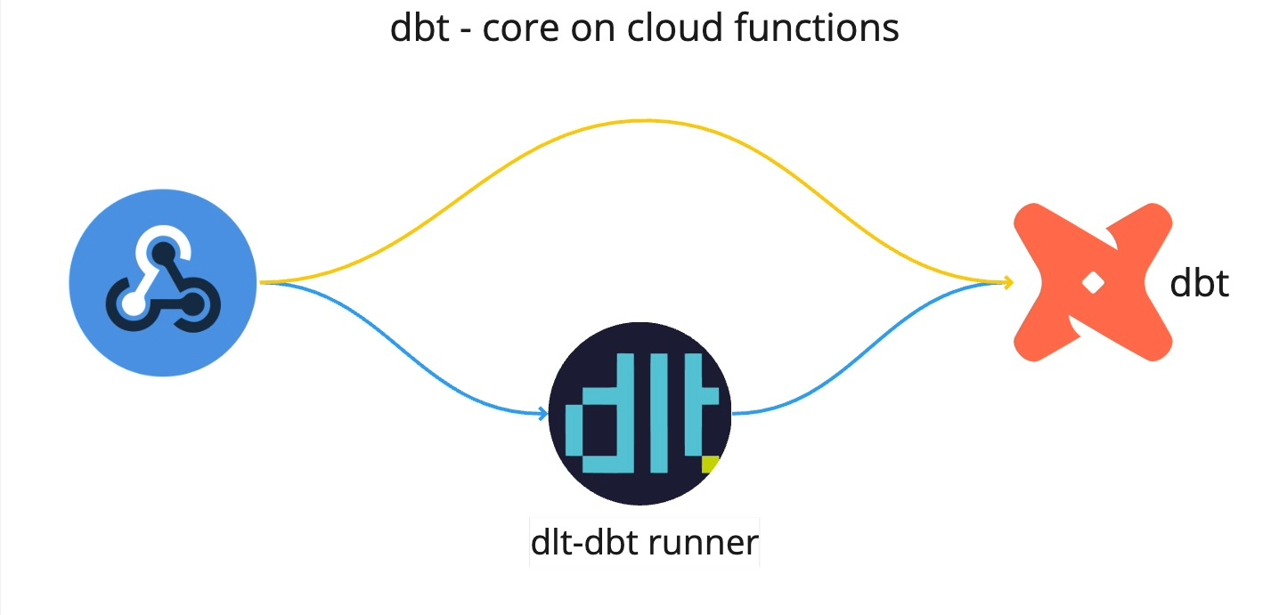
The second option is running dbt using data load tool(dlt).
I work at dlthub and often create dlt pipelines. These often need dbt for modeling the data, making
the dlt-dbt combination highly effective. For using this combination on cloud functions, we used
dlt-dbt runner developed
at dlthub.
The main reason I use this runner is because I load data with dlt and can re-use dlt’s connection to
the warehouse to run my dbt package, saving me the time and code complexity I’d need to set up and
run dbt standalone.
To integrate dlt and dbt in cloud functions, use the dlt-dbt runner; here’s how:
Lets start by creating the following directory structure:
You can set up the dbt by initing a new project, for details refer to
documentation.
note
With the dlt-dbt runner configuration, setting up a profiles.yml is unnecessary. DLT seamlessly
shares credentials with dbt, and on Google Cloud Functions, it automatically retrieves service
account credentials, if none are provided.
Next, configure the dbt_projects.yml and set the model directory, for example:
model-paths:["dbt_transform/models"]
Next, configure the main.py as follows:
import dlt import logging, json from flask import jsonify from dlt.common.runtime.slack import send_slack_message defrun_pipeline(request): """ Set up and execute a data processing pipeline, returning its status and model information. This function initializes a dlt pipeline with pre-defined settings, runs the pipeline with a sample dataset, and then applies dbt transformations. It compiles and returns the information about each dbt model's execution. Args: request: The Flask request object. Not used in this function. Returns: Flask Response: A JSON response with the pipeline's status and dbt model information. """ try: # Sample data to be processed data =[{"name":"Alice Smith","id":1,"country":"Germany"}, {"name":"Carlos Ruiz","id":2,"country":"Romania"}, {"name":"Sunita Gupta","id":3,"country":"India"}] # Initialize a dlt pipeline with specified settings pipeline = dlt.pipeline( pipeline_name="user_data_pipeline", destination="bigquery", dataset_name="dlt_dbt_test" ) # Run the pipeline with the sample data pipeline.run(data, table_name="sample_data") # Apply dbt transformations and collect model information models = transform_data(pipeline) model_info =[ { "model_name": m.model_name, "time": m.time, "status": m.status, "message": m.message } for m in models ] # Convert the model information to a string model_info_str = json.dumps(model_info) # Send the model information to Slack send_slack_message( pipeline.runtime_config.slack_incoming_hook, model_info_str ) # Return a success response with model information return jsonify({"status":"success","model_info": model_info}) except Exception as e: # Log and return an error response in case of any exceptions logging.error(f"Error in running pipeline: {e}", exc_info=True) return jsonify({"status":"error","error":str(e)}),500 deftransform_data(pipeline): """ Execute dbt models for data transformation within a dlt pipeline. This function packages and runs all dbt models associated with the pipeline, applying defined transformations to the data. Args: pipeline (dlt.Pipeline): The pipeline object for which dbt transformations are run. Returns: list: A list of dbt model run information, indicating the outcome of each model. Raises: Exception: If there is an error in running the dbt models. """ try: # Initialize dbt with the given pipeline and virtual environment dbt = dlt.dbt.package( pipeline, "/workspace/dbt_transform", venv=dlt.dbt.get_venv(pipeline) ) logging.info("Running dbt models...") # Run all dbt models and return their run information return dbt.run_all() except Exception as e: # Log and re-raise any errors encountered during dbt model # execution logging.error(f"Error in running dbt models: {e}", exc_info=True) raise # Main execution block if __name__ =="__main__": # Execute the pipeline function. run_pipeline(None)
The send_slack_message function is utilized for sending messages to Slack, triggered by
both success and error events. For setup instructions, please refer to the official
documentation here.
RUNTIME__SLACK_INCOMING_HOOK was set up as environment variable in the above code.
Next, list runtime-installable modules in requirements.txt:
dbt-core
dbt-bigquery
Finally, you can deploy the function using gcloud CLI as:
The merit of this method is that it can be used to load and transform data simultaneously. Using dlt
for data loading and dbt for modeling makes using dlt-dbt a killer combination for data engineers
and scientists, and my preferred choice. This method is especially effective for batched data and
event-driven pipelines with small to medium workloads. For larger data loads nearing timeout limits,
consider separating dlt and dbt into different cloud functions.
Deployment considerations: How does cloud functions compare to Git Actions?
At dlthub we already natively support deploying to GitHub Actions, enabling you to have a serverless setup with a 1-command deployment.
GitHub actions is an orchestrator that most would not find suitable for a data warehouse setup - but
it certainly could do the job for a minimalistic setup. GitHub actions provide 2000 free minutes per
month, so if our pipelines run for 66 minutes per day, we fit in the free tier. If our pipelines
took another 1h per day, we would need to pay ~15 USD/month for the smallest machine (2 vCPUs) but you
can see how that would be expensive if we wanted to run it continuously or had multiple pipelines always-on in parallel.
Cloud functions are serverless lightweight computing solutions that can handle small computational
workloads and are cost-effective. dbt doesn't require the high computing power of the machine
because it uses the computing power of the data warehouse to perform the transformations. This makes
running dbt-core on cloud functions a good choice. The free tier would suffice for about 1.5h per
day of running a 1 vCPU and 2 GB RAM machine, and if we wanted an additional 1h
per day for this hardware it would cost us around 3-5 USD/month.
When deploying dbt-core on cloud functions, there are certain constraints to keep in mind. For instance,
there is a 9-minute time-out limit for all 1st Gen functions. For 2nd Gen functions, there is a 9-minute
limit for event-driven functions and a 60-minute limit for HTTP functions. Since dbt works on the processing
power of the data warehouse it's operating on, 60 minutes is sufficient for most cases with small to medium
workloads. However, it is important to remember the 9-minute cap when using event-driven functions.
When creating lightweight pipelines, using the two tools together on one cloud function makes a lot
of sense, simplifying the setup process and the handover between loading and transformation.
However, for more resource-intensive pipelines, we might want to improve resource utilisation by
separating the dlt loading from the dbt running because while dbt’s run speed is determined by the
database, dlt can utilize the cloud function’s hardware resources.
When it comes to setting up just a dbt package to run on cloud functions, I guess it comes to
personal preference: I prefer dlt as it simplifies credential management. It automatically shares
credentials with dbt, making setup easier. Streamlining the process further, dlt on Google Cloud
functions, efficiently retrieves service account credentials, when none are provided. I also
used dlt’s Slack error reporting function
that sends success and error notifications from your runs directly to your Slack channel,
helping me manage and monitor my runs.
Empowering people by making data work simple - a value dlt embodies, and so does Mode. Both tools enable a person to build powerful things “on-the-fly”. Hence, when Mode positions itself as a self-service analytics platform, it delivers on that commitment by offering a user-friendly and familiar interface, and holistic experience.
👨🏻🦰, 👨🏻🦱, and 🧕🏻 from Logistics need to know what happened on the 1st of August, now!
The sad story of most data and analytics teams are as follows: they are frequently burdened with routine (or ad-hoc) data requests, often involving simple SQL commands exported to Excel for external use. Despite the apparent simplicity, handling multiple requests simultaneously creates unnecessary workload. This detracts from the analytics team's capacity to engage in more constructive tasks such as cohort analysis, predictive analysis, hypothesis testing, creating funky plots - the fun stuff!
Nevertheless, employees outside the data team should not be blamed for making data requests without meaningful access to the data. If they were empowered to access and utilize the necessary data independently, individuals like 👨🏻🦰, 👨🏻🦱, and 🧕🏻 could filter user data from August 1st without relying on analysts.
Don’t know where you stand as a company, with data? Ask Mode
You can start your company’s journey with Mode by utilizing their data maturity test. It will tell you where you stand on your data democracy practices. A quick survey of user experiences showed exactly how Mode empowered companies of different sizes to become data thinkers. It has been adopted into 50% of Fortune 500 companies already!
Contrary to common belief, fostering a company-wide embrace of data thinking doesn't necessarily entail teaching everyone programming or conducting data science courses. Mode identifies four pivotal factors—people, processes, culture, and tools—that can empower companies to cultivate data thinkers. However, there are more reasons contributing to Mode's success in facilitating the emergence of company-wide "data heroes”. Let’s explore them.
Whether intentional or not, the table view on Mode, alongside by its green and white interface, evokes a sense of familiarity to original BI tool:Excel. Additionally, the platform offers the flexibility of having an SQL-only space and extending that functionality to incorporate Python (and R), providing a user experience similar to utilizing Databricks’ notebook & SQL environment. Lastly, the interface of the dashboarding spaces are the (simplified) experiences of tools like Power BI or Tableau.
When a tool feels familiar, people might embrace it faster. In Mode, all these familiar experiences are combined and simplified into one platform, and this holistic offering could be why Mode is: 1) easy to use and attracts users, and 2) easy to adopt across a company.
Talking about company-wide adoption of a data tool, Mode offers various levels of access tailored to different user roles.
This aligns with the idea behind data democracy, ensuring that individuals throughout the company can engage with data. In Mode, this includes both viewing reports and deriving insights from them, and also viewing the underlying data collection (or datasets). Notably, access can be fine-tuned based on user distinctions, such as developers and business users. This is accomplished through nuanced permission settings and user grouping. By defining specific permissions, one can specify the actions users are empowered to perform. Now, let's explore the specific depth of what these users can actually do with all this power, in the next sections.
Mode stores in itself “datasets”. This goes one step beyond writing a bajillion queries with joins and either saving them as code or saving them as materialized views in your database. You can use SQL and create datasets that are reusable and power a variety of different reports.
Contrast this with the user experience offered by other BI tools, even though they do offer the workspace for table creation, they lack robust documentation and centralization of these tables. It then becomes challenging for other teams (and in a couple of months, yourself) to comprehend the purpose and content of these tables - let alone use them across different reports.
There's no need to switch to a different database engine environment for SQL writing; Mode provides this functionality within its own environment. While tools like Databricks also offer this feature, Mode stands out by seamlessly utilizing it to generate shareable reports, much like the functionality seen in Metabase. Moreover, Mode goes a step further with its integration of Python and R, a capability present in Power BI but notably lacking the user-friendly interface of Mode's notebook environment.
In creating these replicable datasets that can be accessed through different ways, Mode creates a single source of truth. This eliminates the need to search for disparate queries, streamlining the data retrieval (and access) process.
When we discuss data centralization, it typically involves cloud-hosted data warehouses that are accessible to authorized users at any time. This concept extends to business intelligence (BI) as well. Analysts within a company may utilize various tools, different source tables and SQL implementations, such as Apache Superset for business users, and Presto SQL for BI developers in their exploration, this leads to differences in loading and accessing data. Mode, in positioning itself as a central hub for data, resolves this by ensuring uniformity – everyone interacts with the same data source, eliminating variations in querying methods and results.
Speaking of running around for different definitions, we come to the importance of the semantic layer in a data workflow.
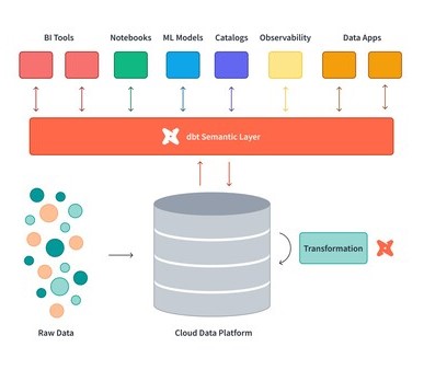
In 2022, dbt introduced its semantic layer to address the challenge faced by BI developers and other stakeholders alike, in standardizing metric and indicator definitions across a company. This aimed to resolve issues arising from different individuals querying and defining these metrics, a process prone to human error (or logical code error) that can lead to inconsistencies. The significance of company-wide metrics lies in their impact on investors and their role in guiding teams on measuring growth and determining actions based on that growth.
This concept bears some resemblance to the centralized metrics approach described here. However it is integrated into data products, its significance remains crucial. Therefore, incorporating dbt into your pipeline and linking it with Mode can significantly contribute to your journey of data centralization and governance.
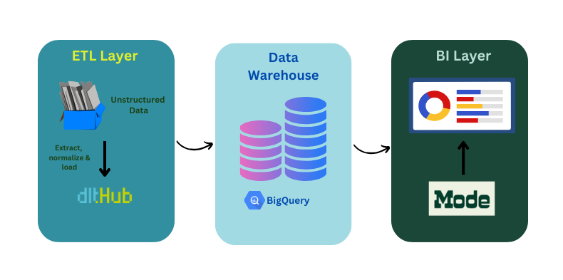
Both dlt and Mode share the core value of data democracy, a cornerstone of the Modern Data Stack. When discussing the modern data stack, we are referring to the integration of various modular components that collaboratively create an accessible central system. Typically, this stack begins with a cloud data warehouse, where data is loaded, and updated by a data pipeline tool, like dlt. This process often involves a transformation layer, such as dbt, followed by the utilization of business intelligence (BI) tools like Mode.
In the context of a Python-based environment, one can employ dlt to ingest data into either a database or warehouse destination. Whether this Python environment is within Mode or external to it, dlt stands as its own independent data pipeline tool, responsible for managing the extract and load phases of the ETL process. Additionally, dlt has the ability to structure unstructured data within a few lines of code - this empowers individuals or developers to work independently.
With simplicity, centralization, and governance at its core, the combination of dlt and Mode, alongside a robust data warehouse, establishes two important elements within the modern data stack. Together, they handle data pipeline processes and analytics, contributing to a comprehensive and powerful modern data ecosystem.
There are two ways to use dlt and Mode to uncomplicate your workflows.
1. Extract, Normalize and Load with dlt and Visualize with Mode
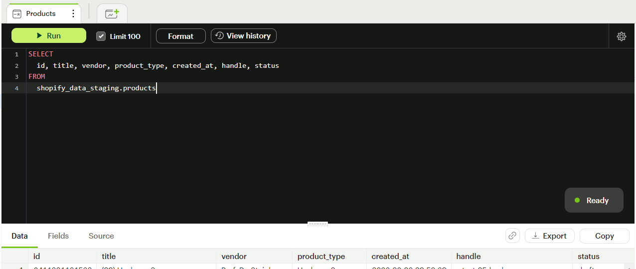
The data we are looking at comes from the source: Shopify. The configuration to initialize a Shopify source can be found in the dltHub docs. Once a dlt pipeline is initialized for Shopify, data from the source can be streamed into the destination of your choice. In this demo, we have chosen for it to be BigQuery destination. From where, it is connected to Mode. Mode’s SQL editor is where you can model your data for reports - removing all unnecessary columns or adding/subtracting the tables you want to be available to teams.
This stage can be perceived as Mode’s own data transformation layer, or semantic modelling layer, depending on which team/designation the user belongs to. Next, the reporting step is also simplified in Mode.
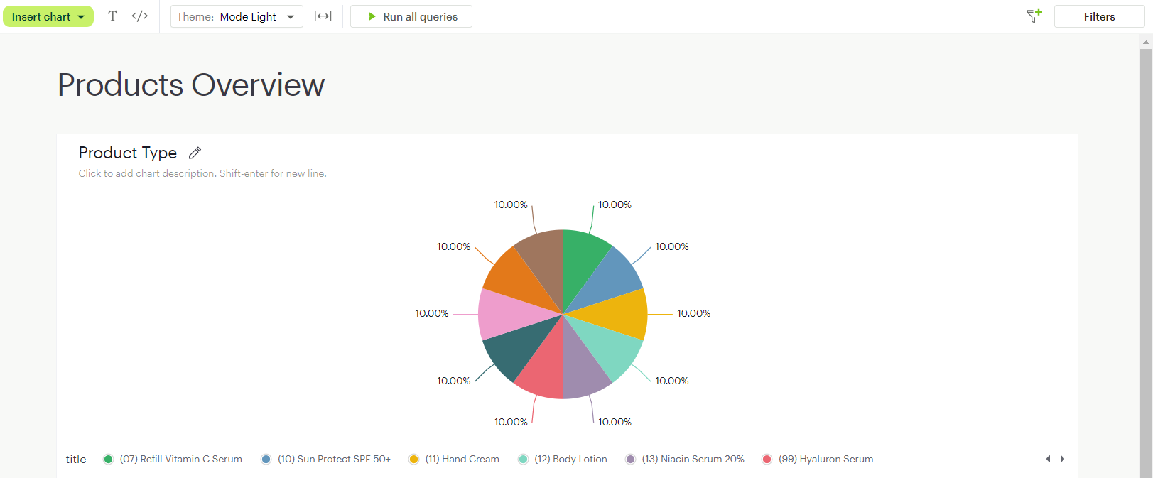
With the model we just created, called Products, a chart can be instantly created and shared via Mode’s Visual Explorer. Once created, it can easily be added to the Report Builder, and added onto a larger dashboard.
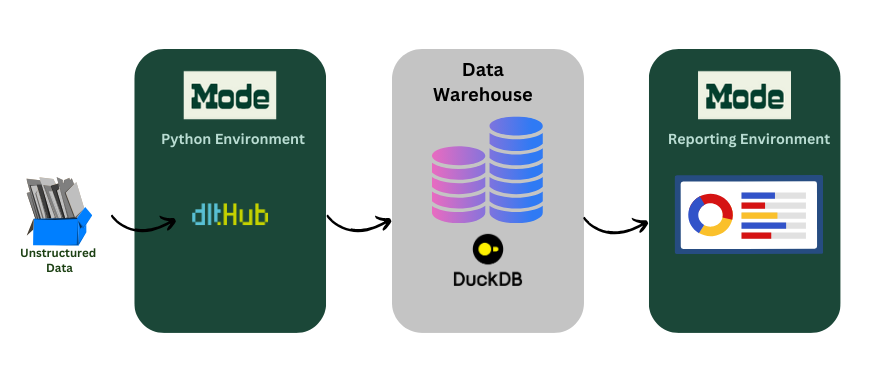
2. Use dlt from within the python workspace in Mode
In this demo, we’ll forego the authentication issues of connecting to a data warehouse, and choose the DuckDB destination to show how the Python environment within Mode can be used to initialize a data pipeline and dump normalized data into a destination. In order to see how it works, we first install dlt[duckdb] into the Python environment.
!pip install dlt[duckdb]
Next, we initialize the dlt pipeline:
# initializing the dlt pipeline with your
# data warehouse destination
pipeline = dlt.pipeline(
        pipeline_name="mode_example_pipeline",
        destination="duckdb",
        dataset_name="staging_data")
And then, we pass our data into the pipeline, and check out the load information. Let's look at what the Mode cell outputs:
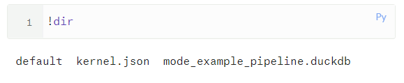
Let’s check if our pipeline exists within the Mode ecosystem:
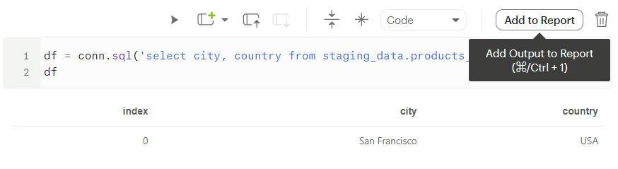
Here we see the pipeline surely exists. Courtesy of Mode, anything that exists within the pipeline that we can query through Python can also be added to the final report or dashboard using the “Add to Report” button.
Once a pipeline is initialized within Mode’s Python environment, the Notebook cell can be frozen, and every consecutive run of the notebook can be a call to the data source, updating the data warehouse and reports altogether!
dlt and Mode can be used together using either method, and make way for seamless data workflows. The first method mentioned in this article is the more traditional method of creating a data stack, where each tool serves a specific purpose. The second method, however utilizes the availability of a Python workspace within Mode to also serve the ETL process within Mode as well. This can be used for either ad-hoc reports and ad hoc data sources that need to be viewed visually, or, can be utilized as a proper pipeline creation and maintenance tool.
TL;DR: William, a gcp data consultant, shares an article about the work he did with dlt and GCP to create a secure, scalable, lightweight, and powerful high-volume event ingestion engine.
He explores several alternatives before offering a solution, and he benchmarks the solution after a few weeks of running.
In the ever-evolving landscape of cloud computing, optimizing data workflows is
paramount for achieving efficiency and scalability. Even though Google Cloud Platform
offers the powerful Dataflow service to process data at scale, sometimes the simplest solution
is worth a shot.
In cases with a relatively high Pub/Sub volume (>10 messages per second), a pull
subscription with a continuously running worker is more cost-efficient and quicker than
a push subscription. Using a combination of Docker, Instance Templates and Instance
Groups, it is pretty simple to set up an auto-scaling group of instances that will
process Pub/Sub messages.
This guide will walk you through the process of configuring GCP infrastructure that
efficiently pulls JSON messages from a Pub/Sub subscription, infers schema, and inserts
them directly into a Cloud SQL PostgreSQL database using micro-batch processing.
The issue at hand
In my current role at WishRoll, I was faced with the issue of processing a high amount
of events and store them in the production database directly.
Imagine the scene: the server application produces analytics-style events such as "user
logged-in", and "task X was completed" (among others). Eventually, for example, we want
to run analytics queries on those events to count how many times a user logs in to
better tailor their experience.
The trivial solution is to synchronously insert these events directly in the database. A
simple implementation would mean that each event fired results in a single insert to the
database. This comes with 2 main drawbacks:
Every API call that produces an event becomes slower. I.e. the /login endpoint needs to insert a record in the database
The database is now hit with a very high amount of insert queries
With our most basic need of 2 event types, we were looking at about 200 to 500 events
per second. I concluded this solution would not be scalable. To make it so, 2 things
would be necessary: (1) make the event firing mechanism asynchronous and (2) bulk events
together before insertion.
A second solution is to use a Pub/Sub push subscription to trigger an HTTP endpoint when
a message comes in. This would've been easy in my case because we already have a
worker-style autoscaled App Engine service that could've hosted this. However, this only
solves the 1st problem of the trivial solution; the events still come in one at a
time to the HTTP service.
Although it's possible to implement some sort of bulking mechanism in a push endpoint,
it's much easier to have a worker pull many messages at once instead.
C. The serverless, fully-managed Dataflow solution
This led me to implement a complete streaming pipeline using GCP's streaming service:
Dataflow. Spoiler: this was way overkill and led to weird bugs with DLT (data load
tool). If you're curious, I've open-sourced that code
too.
This solved both issues of the trivial solution, but proved pretty expensive and hard to
debug and monitor.
Disclaimer: I had never considered standalone machines from cloud providers (AWS EC2, GCP Compute
Engine) to be a viable solution to my cloud problems. In my head, they seemed like
outdated, manually provisioned services that could instead be replaced by managed
services.
But here I was, with a need to have a continuously running worker. I decided to bite the
bullet and try my luck with GCP Compute Engine. What I realized to my surprise, is that
by using instance templates and instance groups, you can easily set up a cluster of workers
that will autoscale.
The code is simple: run a loop forever that pulls messages from a Pub/Sub subscription,
bulk the messages together, and then insert them in the database. Repeat.
Then deploy that code as an instance group that auto-scales based on the need to process
messages.
The pulling and batching logic to accumulate and group messages from Pub/Sub based on
their destination table
The load logic to infer the schema and bulk insert the records into the database. This
part leverages DLT for destination compatibility and schema inference
By using this micro-batch architecture, we strive to maintain a balance of database
insert efficiency (by writing multiple records at a time) with near real-time insertion
(by keeping the window size around 5 seconds).
pipeline = dlt.pipeline( pipeline_name="pubsub_dlt", destination=DESTINATION_NAME, dataset_name=DATASET_NAME, ) pull = StreamingPull(PUBSUB_INPUT_SUBCRIPTION) pull.start() try: while pull.is_running: bundle = pull.bundle(timeout=WINDOW_SIZE_SECS) iflen(bundle): load_info = pipeline.run(bundle.dlt_source()) bundle.ack_bundle() # pretty print the information on data that was loaded print(load_info) else: print(f"No messages received in the last {WINDOW_SIZE_SECS} seconds") finally: pull.stop()
Using DLT has the major advantage of inferring the schema of your JSON data
automatically. This also comes with some caveats:
The output schema of these analytics tables might change based on events
If your events have a lot of possible properties, the resulting tables could become
very wide (lots of columns) which is not something desirable in an OLTP database
Given these caveats, I make sure that all events fired by our app are fully typed and
limited in scope. Moreover, using the table_name_data_key configuration of the code I
wrote, it's possible to separate different events with different schemas into different
tables.
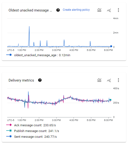
The Pub/Sub subscription metrics. Message throughput ranges between 200 and 300
per second, while the oldest message is usually between 5 and 8 seconds with occasional spikes.
I am running a preemptible (SPOT) instance group of n1-standard-1 machines that
auto-scales between 2 and 10 instances. In normal operation, a single worker can handle
our load easily. However, because of the preemptible nature of the instances, I set the
minimum number to 2 to avoid periods where no worker is running.
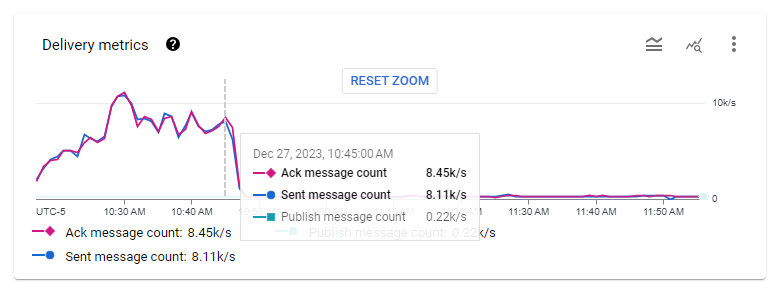
When deploying the solution with a backlog of messages to process (15 hours worth of
messages), 10 instances were spawned and cleared the backlog in about 25 minutes.
The Pub/Sub subscription throughput metrics when a 15-hour backlog was cleared. The
instance group gradually reached 10 instances at about 10:30AM, then cleared the
backlog by 10:50AM.
Between 7000 and 10000 messages per second were processed on average by these 10
instances, resulting in a minimum throughput capacity of 700 messages/s per worker.
Using n1-standard-1 spot machines, this cluster costs $8.03/mth per active machine. With
a minimum cluster size of 2, this means $16.06 per month.
Conclusion
Using more "primitive" GCP services around Compute Engine provides a straightforward and
cost-effective way to process a high throughput of Pub/Sub messages from a pull
subscription.
info
PS from dlt team:
We just added data contracts enabling to manage schema evolution behavior.
Are you on aws? Check out this AWS SAM & Lambda event ingestion pipeline here.
This demo works on codespaces. Codespaces is a development environment available for free to anyone with a Github account. You'll be asked to fork the demo repository and from there the README guides you with further steps.
Welcome to "Codex Central", your next-gen help center, driven by OpenAI's GPT-4 model. It's more than just a forum or a FAQ hub – it's a dynamic knowledge base where coders can find AI-assisted solutions to their pressing problems. With GPT-4's powerful comprehension and predictive abilities, Codex Central provides instantaneous issue resolution, insightful debugging, and personalized guidance. Get your code running smoothly with the unparalleled support at Codex Central - coding help reimagined with AI prowess.